Combine Data From Multiple Worksheets into a Single Worksheet in Excel
I recently got a question from a reader about combining multiple worksheets in the same workbook into one single worksheet.
I asked him to use Power Query to combine different sheets, but then I realized that for someone new to Power Query, doing this can be tough.
So I decided to write this tutorial and show the exact steps to combine multiple sheets into one single table using Power Query.
Below a video where I show how to combine data from multiple sheets/tables using Power Query:
Note: Power Query can be used as an add-in in Excel 2010 and 2013, and is an inbuilt feature from Excel 2016 onwards. Based on your version, some images may look different (image captures used in this tutorial are from Excel 2016).
Combine Data from Multiple Worksheets Using Power Query
When combining data from different sheets using Power Query, it’s required to have the data in an Excel Table (or at least in named ranges). If the data is not in an Excel Table, the method shown here would not work.
Suppose you have four different sheets – East, West, North, and South.
Each of these worksheets has the data in an Excel Table, and the structure of the table is consistent (i.e., the headers are same).
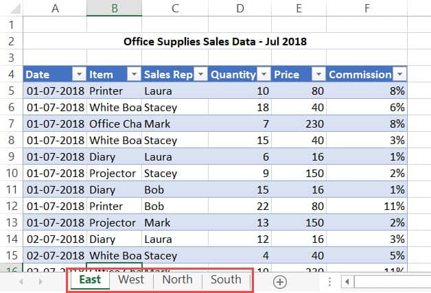
This kind of data is extremely easy to combine using Power Query (which works really well with data in Excel Table).
For this technique to work best, it’s better to have names for your Excel Tables (work without it too, but it’s easier to use when the tables are named).
I have given the tables the following names: East_Data, West_Data, North_Data, and South_Data.
Here are the steps to combine multiple worksheets with Excel Tables using Power Query:
- Go to the Data tab.

- In the Get & Transform Data group, click on the ‘Get Data’ option.

- Go the ‘From Other Sources’ option.
- Click the ‘Blank Query’ option. This will open the Power Query editor.

- In the Query editor, type the following formula in the formula bar: =Excel.CurrentWorkbook(). Note that the Power Query formulas are case sensitive, so you need to use the exact formula as mentioned (else you will get an error).

- Hit the Enter key. This will show you all the table names in the entire workbook (it will also show you the named ranges and/or connections in case it exists in the workbook).

- [Optional Step] In this example, I want to combine all the tables. If you want to combine specific Excel Tables only, then you can click the drop-down icon in the name header and select the ones you want to combine. Similarly, if you have named ranges or connections, and you only want to combine tables, you can remove those named ranges as well.
- In the Content header cell, click on the double pointed arrow.
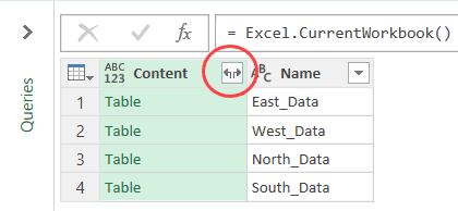
- Select the columns that you want to combine. If you want to combine all columns, make sure (Select All Columns) is checked.
- Uncheck the ‘Use original column name as prefix’ option.

- Click OK.
The above steps would combine the data from all the worksheets into one single table.
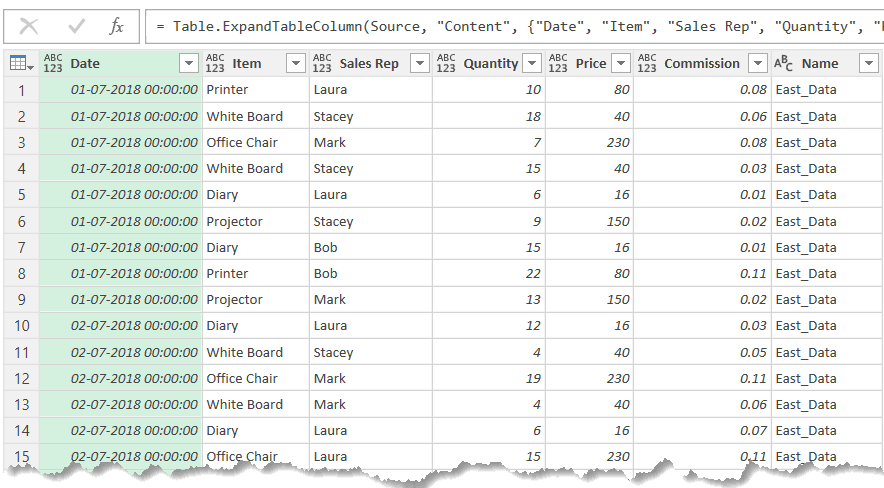
If you look closely, you’ll find the last column (rightmost) has the name of the Excel tables (East_Data, West_Data, North_Data, and South_Data). This is an identifier that tells us which record came from which Excel Table. This is also the reason I said it’s better to have descriptive names for the Excel tables.
Here are a few modifications you can do to the combined data in Power Query itself:
- Drag and place the Name column to the beginning.
- Remove the “_Data” from the name column (so you’re left with East, West, North, and South in the name column). To do this, right-click on the Name header and click on Replace Values. In the Replace Values dialog box, replace _Data with a blank.
- Change the Data column to show only dates (and not the time). To do this, click the Date column header, go to the ‘Transform’ tab and change the Data type to Date.
- Rename the Query to ConsolidatedData.
Now that you have the combined data from all the worksheets in Power Query, you can load it in Excel – as a new table in a new worksheet.
To do this. follow the below steps:
- Click the ‘File’ tab.
- Click on Close and Load To.

- In the Import Data dialog box, select Table and New worksheet options.

- Click Ok.
The above steps would combine data from all the worksheets and give you that combined data in a new worksheet.
One Issue You Must Resolve when Using This Method
In case you have used the above method to combine all the tables in the workbook, you’re likely to face an issue.
See the number of rows of the combined data – 1304 (which is right).
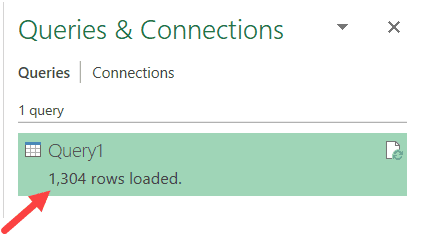
Now, if I refresh the query, the number of rows changes to 2607. Refresh again and it will change to 3910.
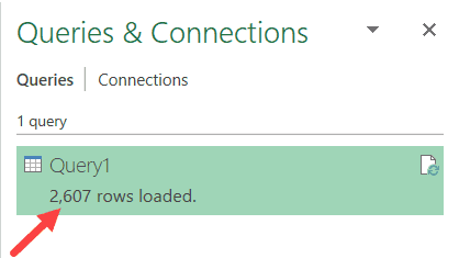
Here is the problem.
Every time you refresh the query, it adds all the records in the original data to the combined data.
Let’s understand the cause of this problem and how to correct this.
When you refresh a query, it goes back and follows all the steps that we took to combine the data.
In the step where we used the formula =Excel.CurrentWorkbook(), it gave us a list of all the tables. This worked fine the first time as there were only four tables.
But when you refresh, there are five tables in the workbook – including the new table that Power Query inserted where we have the combined data.
So every time you refresh the query, apart from the four Excel Tables that we want to combine, it also adds the existing query table to the resulting data.
This is called recursion.
Here is how to solve this issue.
Once you insert =Excel.CurrentWorkbook() in the Power Query formula bar and hit enter, you get a list of Excel Tables. To make sure you only get to combine the tables from the worksheet, you need to somehow filter only these tables that you want to combine and remove everything else.
Here are the steps to make sure you only have the required tables:
- Click the drop-down and hover the cursor on Text Filters.
- Click on the Contains option.
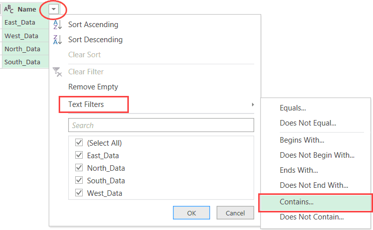
- In the Filter Rows dialog box, enter _Data in the field next to the ‘contains’ option.

- Click OK.
You may not see any change in the data, but doing this will prevent the resulting table from being added over again when the query is refreshed.
Note that in the above steps we have used “_Data” to filter as we named out tables that way. But what if your tables are not named consistently. What if all the table names are random and have nothing in common.
Here is the way to solve this – use the ‘does not equal’ filter and enter the name of the Query (which would be ConsolidatedData in our example). This will ensure that everything remains the same and the resulting query table which is created is filtered out.
Important Note: In the example used in this tutorial, the headers were same. In case the headers are different, Power Query will combine and create all the columns in the new table. If the data is available for that column, it will be shown, else it will show null.
#evba #etipfree #kingexcel📤You download App EVBA.info installed directly on the latest phone here : https://www.evba.info/p/app-evbainfo-setting-for-your-phone.html?m=1


![[Free ebook Download]Excel Formulas & Functions For Dummies by Ken Bluttman](https://blogger.googleusercontent.com/img/b/R29vZ2xl/AVvXsEhYetQg74WpM626jRfy2FNrD3T272FyEaS-6p2mBfAgithEES51mLuj76s7JDCrkb8SuwiaST1s6mox68MC6IwJYWkiFH6rRXYqnc513XGjRdYjeviLZii14QmxmThmh2D_ItCW1YTvd2k/s72-c/Excel+Formulas+%2526+Functions+For+Dummies+by+Ken+Bluttman.jpg)
![[FREE EBOOK DOWNLOAD]Excel Data Analysis For Dummies by Paul McFedries](https://blogger.googleusercontent.com/img/b/R29vZ2xl/AVvXsEgLCDTLwgLtY0xfs-YAIKyDdKhMVSIKsrnjL-GtIYwV7BD7oqVTMWc3cTR73ps7GtjNrZB5v84xN5ROGdf9_YW1oeTiV4mgMeIdfV7LZOiEBbJuY15C7Qch4jNUYd6Eb3oE_xmQUSrdfCI/s72-c/Excel+Data+Analysis+For+Dummies+by+Paul+McFedries.jpg)
![[Free ebook] Excel Timesaving Techniques For Dummies](https://blogger.googleusercontent.com/img/b/R29vZ2xl/AVvXsEgzWyqaPosaS2VM-Nk1ab24vcKUwYTs711ThM9wp9xmavw0A3qGwRFO810Ck-OdOWZcBBky6MTqkpWRXlaZBidjaesv3AhqgLAVXQ-jUZj8erqehdQDFbSg8s0XB72D162a5fdjoeCaXCU/s72-c/2019_04_15_14.32.34_edit.jpg)
![[FREE EBOOK]101 Ready-to-Use Excel Formulas by Michael Alexander & Dick Kusleika](https://blogger.googleusercontent.com/img/b/R29vZ2xl/AVvXsEjlgcYWkmfYQbPJ8_2JubQnnsTSWEba0oUXWpGF53A6EOj30ZsVldkShWT3woS6WnNIDHMuTkRGl2Fnj8e86GA7-PRE1HEhKN6Yw_gJe00lzcxRpCXafd4IRO97ehk3PNQybVPn3k4q7r8/s72-c/101+Ready-to-Use+Excel+Formulas+by+Michael+Alexander+%2526+Dick+Kusleika.jpg)

![[Free ebook]John Charnes – Financial Modeling with Crystal Ball & Excel](https://blogger.googleusercontent.com/img/b/R29vZ2xl/AVvXsEiPP0330djpk28pL5LZlqnuEaIplflr5MdFS78ohWpHrWhis4Fy49pyqGS3jAqINNEwiqnNifTCRJgTlxVr5wJfaozf7SUX_tFXmD9grSAoXyOyZQjt2GdaryCkMlqJW0B3NAujFatY7gw/s72-c/395-1.jpg)

![[Free ebook]Excel Dashboards and Reports for Dummies 3rd Edition - Michael Alexander](https://blogger.googleusercontent.com/img/b/R29vZ2xl/AVvXsEh9vLm6q3B9PFEAcLnQ4YrI5pH_KCv-CcunxTBBHZXcbA9rhd2RR2HchlVAguPCGRJupUJesFUkaff2DX7MCqOFwfLHU6LkePD5KMPLZB6V_9Xe64x9p_ntwaFpJMAsjYPaL1sUVMwzhuc/s72-c/2020_01_20_22.10.34_edit.jpg)

No comments:
Post a Comment