Troubleshoot VLOOKUP

Sunday, January 26, 2020 Excel tips, Function in Excel,

Troubleshoot VLOOKUP

VLOOKUP is my favorite function in Excel. If you can use VLOOKUP, you can solve many problems in Excel. But there are things that can trip up a VLOOKUP. This topic talks about a few of them.

But first, the basics of VLOOKUP in plain English.

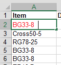
The data in A:C came from the IT department. You asked for sales by item and date. They gave you item number. You need the item description. Rather than wait for the IT department to rerun the data, you find the table shown in column F:G.

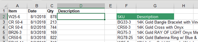
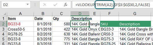
You have a list of item numbers in column A. You need to get the item description from a table in F & G. The table has item number in F and Description in G.

You want VLOOKUP to find the item in A2 while it searches through the first column of the table in $F$3:$G$30. When VLOOKUP finds the match in F7, you want VLOOKUP to return the description found in the second column of the table. Every VLOOKUP that is looking for an exact match has to end in False (or zero, which is equivalent to False). The formula below is set up properly.

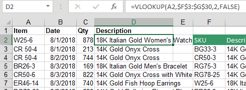
The formula is =VLOOKUP(A2,$F$3:$G$30,2,False)

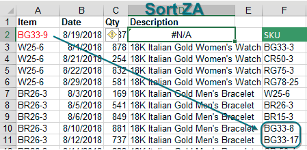
Notice that you use F4 to add four dollar signs to the address for the lookup table. As you copy the formula down column D, you need the address for the lookup table to remain constant. There are two common alternatives: You could specify the entire columns F:G as the lookup table. Or, you could name F3:G30 with a name such as ItemTable. If you use =VLOOKUP(A2,ItemTable,2,False), the named range acts like an absolute reference.

Any time you do a bunch of VLOOKUPs, you need to sort the column of VLOOKUPs. Sort ZA, and any #N/A errors come to the top. In this case, there is one. Item BG33-9 is missing from the lookup table. Maybe it is a typo. Maybe it is a brand-new item. If it is new, insert a new row anywhere in the middle of your lookup table and add the new item.

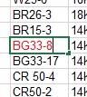
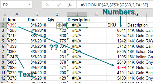
Sort the original data by the VLOOKUP column descending. Any #N/A errors will come to the top of the data set.

It is fairly normal to have a few #N/A errors. But in the figure below, exactly the same formula is returning nothing but #N/A. When this happens, see if you can solve the first VLOOKUP. You are looking up the BG33-8 found in A2. Start cruising down through the first column of the lookup table. As you can see, the matching value clearly is in F10. Why can you see this, but Excel cannot see it?

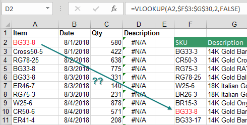
Here, the correct VLOOKUP formula is returning #N/A to every cell. The screenshot is showing that the first item number is very clearly in the lookup table.

Go to each cell and press the F2 key. The figure below shows F10. Note that the insertion cursor appears right after the 8.

Cell F10 is in edit mode, you can see the flashing insertion cursor right after the last character of the part number.

The following figure shows cell A2 in Edit mode. The insertion cursor is a couple of spaces away from the 8. This is a sign that at some point, this data was stored in an old COBOL data set. Back in COBOL, if the Item field was defined as 10 characters and you typed only 6 characters, COBOL would pad it with 4 extra spaces.

Cell A2 is in edit mode. This time, the flashing insertion point is a few cells away from the last character in the part number. This means there are trailing spaces.

The solution? Instead of looking up A2, look up TRIM(A2).

Change the formula to use TRIM: =VLOOKUP(TRIM(A2),$F$3:$G$30,2,False).

The TRIM() function removes leading and trailing spaces. If you have multiple spaces between words, TRIM converts them to a single space. In the figure below there are spaces before and after both names in A1. =TRIM(A1) removes all but one space in A3.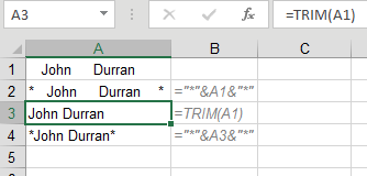

Here is how Trim works: Say that A1 has spaces, then Word1 then several spaces then Word2 then several spaces. =TRIM(A1) will return Word1 Space Word2. While TRIM removes all spaces before the first word and after the last word, it will leave a single space between words.

By the way, what if the problem had been trailing spaces in column F instead of column A? Add a column of TRIM() functions to E, pointing to column F. Copy those and paste as values in F to make the lookups start working again.

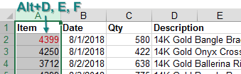
The other very common reason that VLOOKUP won’t work is shown here. Column F contains real numbers. Column A holds text that looks like numbers.

Here is another way VLOOKUP can go wrong. You are looking up a text cell that says 4399 against a table that contains numeric 4399. VLOOKUP will return #N/A instead of the right answer.

Select all of column A. Press Alt+D, E, F. This does a default Text to Columns operation and converts all text numbers to real numbers. The lookup starts working again.

Choose the column of text numbers in column A. Press Alt+D E F. The text numbers convert to numbers and the VLOOKUPs start working again.

If you want the VLOOKUP to work without changing the data, you can use =VLOOKUP(1*A2,...) to handle numbers stored as text or =VLOOKUP(A2&"",...) when your lookup table has text numbers.

#evba #etipfree #kingexcel
📤You download App EVBA.info installed directly on the latest phone here : https://www.evba.info/p/app-evbainfo-setting-for-your-phone.html?m=1