Highlight Rows Between Two Dates with Conditional Formatting in Excel

Bottom Line: Learn to apply conditional formatting for entire rows based on two dates in Excel. Highlight entries within or outside of a date range.

Skill Level: Advanced

Video Tutorial

Download the Excel File

You can download the file that I use in the video in order to follow along.

 Conditional Formatting Between Dates.xlsx (252.1 KB)

Highlighting Rows Based on a Condition

This is the second post in a series about formatting entire rows based on conditions. I recommend you check out this prior post first to get a better understanding of how you can use the data in single cell as the basis for conditionally formatting an entire row:

Highlighting Entries Based on Dates

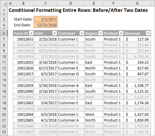
Building on the concept of formatting rows based on cell data, today's post will describe how to highlight rows based on two dates. You can format rows that have an entry between or outside of any two given dates so that they stand out in your table. Here's an example of a sheet that formats rows containing a date anywhere between January 1, 2018, and December 31, 2018.

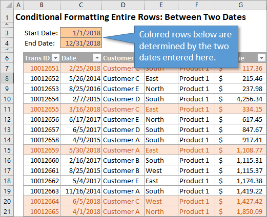
The formatting is both automatic and dynamic. This means that if you change the Start or End Date, the table will instantly update to reflect the change.

Between Two Dates

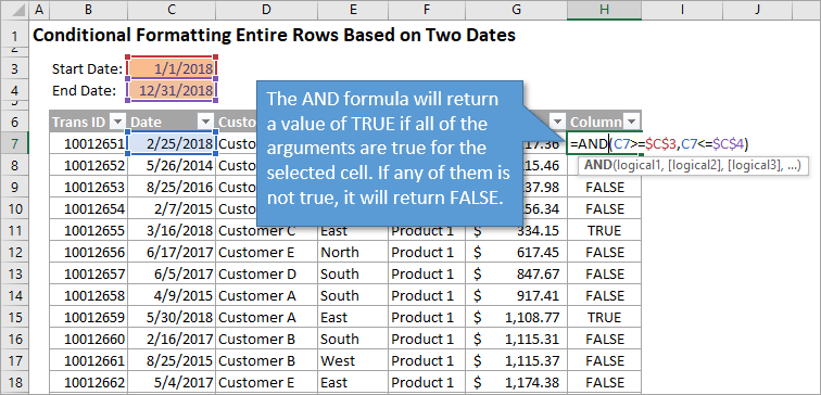
To highlight a row that has a cell that is between two dates, we are going to use the AND function.

The AND function has arguments for two or more logical tests. Each logical test must return a True or False value. This is usually done with comparison operators (=, <, >, <>).

Our first argument will say that the date in the cell we choose must be greater than or equal to (>=) our start date. In our example this looks like C7>=$C$3. (The dollar signs denote that this is an absolute value that won't change when changes are made to the worksheet.)

Our second argument is that the date should be less than or equal to (<=) the end date. C7<=$C$4.

Putting it all together, the formula for our example is: =AND (C7>=$C$3, C7<=$C$4)

Applying the Conditional Formatting

Now that we see how the formula is written, we will apply the formatting. Here are the steps to do that.

1. Select the cell in the first entry of the date column. In my example worksheet, that's column C.
2. On the Home tab of the Ribbon, select the Conditional Formatting drop-down and click on Manage Rules…. That will bring up the Conditional Formatting Rules Manager window.
3. Click on New Rule. This will open the New Formatting Rule window.
4. Under Select a Rule Type, choose Use a formula to determine which cells to format.
5. Under Format values where this formula is true, you are going to write the formula that we created in the section above: =AND ($C7>=$C$3, $C7<=$C$4)
6. When filling in the values while writing the formula, Excel may automatically put the absolute reference indicators in front of C7, so that it looks like $C$7. To ensure that the conditional formatting applies to all of the rows in the table, we need to change the absolute relative referencing. In other words, we are going to remove that dollar sign in front of the row number (7) in our formula. You can either manually delete it, or you can hit F4 twice to accomplish this step.
   
   This means the formula will always use column C for the comparison, but the row number will change as the formula is evaluated in each row of the table.
7. Click on the Format… button to choose whatever format options you like. You can change the font, the fill, the border, etc.

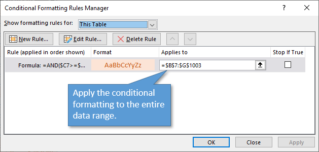
By hitting OK, you'll be taken back to the Conditional Formatting Rules Manager. The only change we want to make here is to include the entire table, not just the cell we started from.

To do that, click on the icon to the right of the Applies to field (it has an upward facing arrow) and select the range of the entire table. In the example, this would be the data ranging from B7 to G1003 (=$B$7:$G$1003).

Outside Two Dates

We've looked at how to identify numbers that fall between two dates, but what if we want to highlight the opposite? We can use the OR function to draw attention to dates that fall outside of a date range (before the start date or after the end date).

The OR function checks whether any of the arguments are true, and if one of them is true, it returns TRUE. They don't have to all be true. Only if all of the arguments are false will the function return FALSE.

Similar to the AND function in the way that it's written, the OR function instead looks for anything less than or equal to (<=) the start date OR greater than or equal (>=) the end date.

So for our example, we will use =OR($C7<=$C$3, $C7>=$C$4)

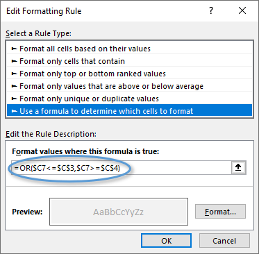
Once that rule is applied, any entry that falls outside of the specified date range will be formatted to stand out.

Conclusion

Both of these techniques also work with regular numbers, not just dates, so keep that in mind.

#evba #etipfree #eama #kingexcel
📤How to Download ebooks: https://www.evba.info/2020/02/instructions-for-downloading-documents.html?m=1