How to Prevent VLOOKUP Errors when Inserting or Deleting Columns
Bottom Line: Learn how to use the COLUMNS function in VLOOKUP to prevent errors when inserting/deleting columns from your source range.
Skill Level: Intermediate
Video Tutorial
Download the Excel File
If you'd like to practice using the COLUMNS function in VLOOKUP using the same data I use in the video, download my file below.
Prevent VLOOKUP Errors When Columns Change
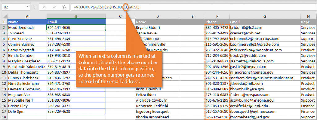
One limitation when using VLOOKUP is that it can easily return the wrong data when the information in the table array gets rearranged. Adding or deleting a column can mess up your data because VLOOKUP uses the column number when it formulates its answer.
For example, in this image below, you can see on the left that we've set up the VLOOKUP formula to return the email address for each of the names listed. The email address is found in the third column of the table array on the right.
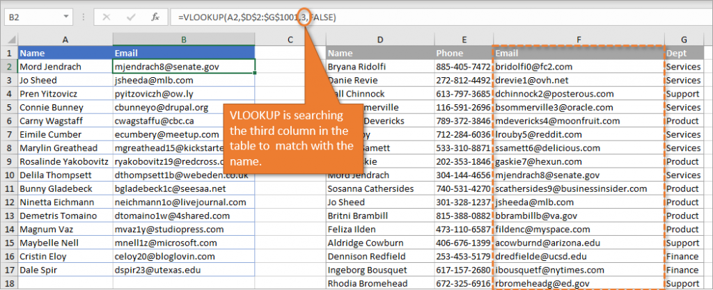
If we add or delete columns and shift those email addresses over, VLOOKUP will continue to return whatever data is found in the that third column.
The COLUMNS Function
There are several ways to fix this problem and the one I'm going to focus on in this tutorial is by using the COLUMNS function. This function returns the number of columns in an array or reference. To use the COLUMNS function just
- Type the equals sign (=) and begin typing the word “Columns.”
- Tab into the COLUMNS function (plural, not singular).
- Select your array. In the example below, I've selected from cell D1 to G1. Because there are four columns in that array (D, E, F, and G), the function returns the value of 4. As I add or delete columns in that array, that value will increase or decrease respectively.
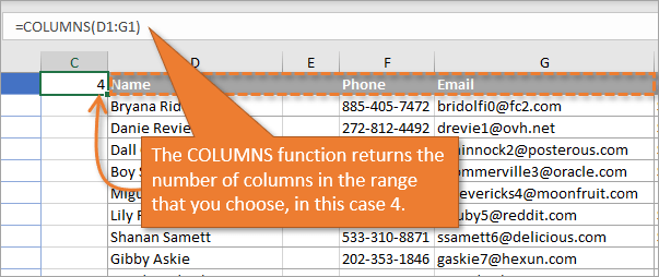
So the COLUMNS function allows our reference to be dynamic. As columns in our range are added or deleted, that number remains the same. The number will identify the data we want because we end our array with the column we are interested in. There may be more columns of data, but we want to end our array with the column we are looking to use.
In our example, no matter how many columns we add or subtract in front of the email column, that column's number will always be the same as the total number of columns in our array (because it's the last column).
Replacing the Column Index Number
This formula that we've created can be used in place of the Column Index Number in our VLOOKUP formula.
One important step when selecting your array is to hit F4, which makes it an absolute reference. (Dollar symbols will be inserted in front of the row and column characters, indicating they are now absolute.)
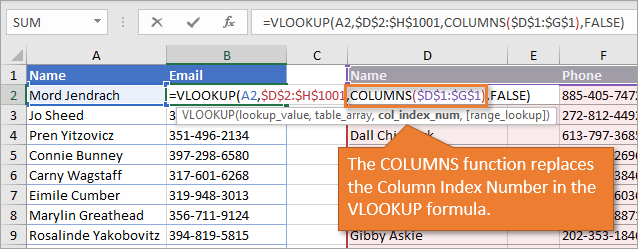
Another good idea is to select the column headers (if there are any) when you are defining your range for the dynamic Column Index Number. That's because additions and deletions might be made to the data in the columns, but the headers are less likely to change.
By the way, the keyboard shortcut to add a column is Ctrl + + and the shortcut to delete a column is Ctrl + -.
Using the COLUMNS Function with Excel Tables
The COLUMNS function also works using ranges that are formatted as Excel Tables. The formula just looks more like this.
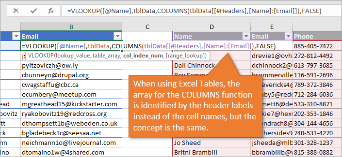
One advantage of using Excel Tables is that you can move columns around (within the existing parameters of the table data) and the VLOOKUP formula will still work correctly.
Pros & Cons
So, to summarize a bit, let me just outline some pros and cons of using the COLUMNS function in your VLOOKUP formula.
Pros
- This option is really easy to implement.
- Updating any existing VLOOKUP formulas is easy as well.
Cons
- The formula can break if columns are moved with regular ranges.
- Although moving columns still works with Excel Tables, you still can’t look to the left, or return a column to the left of the lookup column.
An alternative to avoid these cons is to use INDEX and MATCH and the new XLOOKUP, which you can learn more about in the tutorials outline below.
📤How to Download ebooks: https://www.evba.info/2020/02/instructions-for-downloading-documents.html?m=1


![[FREE EBOOK]101 Ready-to-Use Excel Formulas by Michael Alexander & Dick Kusleika](https://blogger.googleusercontent.com/img/b/R29vZ2xl/AVvXsEjlgcYWkmfYQbPJ8_2JubQnnsTSWEba0oUXWpGF53A6EOj30ZsVldkShWT3woS6WnNIDHMuTkRGl2Fnj8e86GA7-PRE1HEhKN6Yw_gJe00lzcxRpCXafd4IRO97ehk3PNQybVPn3k4q7r8/s72-c/101+Ready-to-Use+Excel+Formulas+by+Michael+Alexander+%2526+Dick+Kusleika.jpg)
![[Free ebook] Excel Timesaving Techniques For Dummies](https://blogger.googleusercontent.com/img/b/R29vZ2xl/AVvXsEgzWyqaPosaS2VM-Nk1ab24vcKUwYTs711ThM9wp9xmavw0A3qGwRFO810Ck-OdOWZcBBky6MTqkpWRXlaZBidjaesv3AhqgLAVXQ-jUZj8erqehdQDFbSg8s0XB72D162a5fdjoeCaXCU/s72-c/2019_04_15_14.32.34_edit.jpg)
![[FREE EBOOK DOWNLOAD]Excel Data Analysis For Dummies by Paul McFedries](https://blogger.googleusercontent.com/img/b/R29vZ2xl/AVvXsEgLCDTLwgLtY0xfs-YAIKyDdKhMVSIKsrnjL-GtIYwV7BD7oqVTMWc3cTR73ps7GtjNrZB5v84xN5ROGdf9_YW1oeTiV4mgMeIdfV7LZOiEBbJuY15C7Qch4jNUYd6Eb3oE_xmQUSrdfCI/s72-c/Excel+Data+Analysis+For+Dummies+by+Paul+McFedries.jpg)
![[Free ebook]Excel Dashboards and Reports for Dummies 3rd Edition - Michael Alexander](https://blogger.googleusercontent.com/img/b/R29vZ2xl/AVvXsEh9vLm6q3B9PFEAcLnQ4YrI5pH_KCv-CcunxTBBHZXcbA9rhd2RR2HchlVAguPCGRJupUJesFUkaff2DX7MCqOFwfLHU6LkePD5KMPLZB6V_9Xe64x9p_ntwaFpJMAsjYPaL1sUVMwzhuc/s72-c/2020_01_20_22.10.34_edit.jpg)
![[Free ebook Download]Excel Formulas & Functions For Dummies by Ken Bluttman](https://blogger.googleusercontent.com/img/b/R29vZ2xl/AVvXsEhYetQg74WpM626jRfy2FNrD3T272FyEaS-6p2mBfAgithEES51mLuj76s7JDCrkb8SuwiaST1s6mox68MC6IwJYWkiFH6rRXYqnc513XGjRdYjeviLZii14QmxmThmh2D_ItCW1YTvd2k/s72-c/Excel+Formulas+%2526+Functions+For+Dummies+by+Ken+Bluttman.jpg)
![[FREE EBOOK]Excel Formulas & Functions For Dummies, 5th Ed. By Ken Bluttman](https://blogger.googleusercontent.com/img/b/R29vZ2xl/AVvXsEjdoqrCzzIOuNJbvUH5MEY1YxOxUOFgEryEJ9qqxXoz_q8tpXdTXpqlw8byu_e9mr68In_O-gqRSMR1BsK6QZu_yNYfUqgEgU0nq3fzjHLngvxWo1xpHMG7TmzBLz3CbjwQT92f8AN2D9c/s72-c/2020_04_13_17.39.05.jpg)
![[Free 7 PDF ebooks]Our Best Excel Cheat Sheets Part 3- 7 Cheat sheets free Download](https://blogger.googleusercontent.com/img/b/R29vZ2xl/AVvXsEgNMjh7jVGVJVBdnE0t2D2xnuAD057LL-Ew6gXJz9LfOId0bd15_tqYhUkdLEkJ8f6kALhG1wvl3klZJhhki1p2edzCel595bAS2vmvIZr60WTVu1lMvaTHED9c2X3e3gJbST-JZRM8CnQ/s72-c/2019_12_23_23.16.18_edit.jpg)

No comments:
Post a Comment